Tutorial: Profiling a PyTorch Model#

In this tutorial, we will use Metinor to profile a PyTorch model. Profiling a model is important to understand the performance of the model and to identify bottlenecks. Metinor provides a simple API to profile a model and a set of tools to analyze and plot the results.

[1]:

# Suppress warnings (to make the output cleaner in this notebook)
import warnings

warnings.filterwarnings("ignore")

Create a model#

The profiler in Metinor supports subclasses of nn.Module. In this tutorial, we will use a pre-trained ResNet-18 from torchvision.

[2]:

from torchvision.models import resnet18, ResNet18_Weights

# Create the model to profile
model = resnet18(weights=ResNet18_Weights.DEFAULT)
input_shape = (3, 224, 224)

Import the profiler#

Next, we will import the profiler from the metinor.profiler package. This is available as metinor.profiler.Profiler class and several metinor.functional.profiler.profile_* functions. We will profile both the model types using the profiler class and the functions.

Profiling a model using the functional API#

[3]:

from nervai_optim.functional.profiler import profile_metrics

# Profile the model
model_report = profile_metrics(model, input_shape=input_shape)

# Report is a `metinor.profiler.ProfileReport` object which contains the following variables:
# - `report.summary`: A summary of the profiled model
# - `report.details`: A layer-by-layer breakdown of the profiled model
# - `report.pretty_summary`: A human-readable summary of the profiled model
# - `report.pretty_details`: A human-readable layer-by-layer breakdown of the profiled model
# Each of these variables is a `pandas.DataFrame` object

# Print the summary of the profiled model
model_report.pretty_summary

[3]:

	ProfilerMetric.NAME	ProfilerMetric.TYPE	ProfilerMetric.INPUTS	ProfilerMetric.OUTPUTS	ProfilerMetric.PARAMS	ProfilerMetric.PARAMS_TRAINABLE	ProfilerMetric.FLOPS	ProfilerMetric.MADDS	ProfilerMetric.MEM_READ	ProfilerMetric.MEM_WRITE	ProfilerMetric.RUNTIME	ProfilerMetric.RMS
0	ResNet	ResNet	(3, 224, 224)	(1000,)	11.69M	11.69M	1.82G	3.64G	18.71M	6.72M	0.028	7.07

[4]:

# Show some details of first 10 layers
from nervai_optim.profiler.metrics import ProfilerMetric

columns = [
    ProfilerMetric.NAME,
    ProfilerMetric.TYPE,
    ProfilerMetric.FLOPS,
    ProfilerMetric.MADDS,
    ProfilerMetric.RUNTIME,
]
model_report.pretty_details[columns].head(10)

[4]:

	ProfilerMetric.NAME	ProfilerMetric.TYPE	ProfilerMetric.FLOPS	ProfilerMetric.MADDS	ProfilerMetric.RUNTIME
1	conv1	Conv2d	118.01M	235.23M	0.0025
2	bn1	BatchNorm2d	1.61M	3.21M	0.0006
3	relu	ReLU	802.82K	802.82K	0.00014
4	maxpool	MaxPool2d	802.82K	1.61M	0.0013
5	layer1.0.conv1	Conv2d	115.61M	231.01M	0.0012
6	layer1.0.bn1	BatchNorm2d	401.41K	802.82K	0.00022
7	layer1.0.relu	ReLU	200.7K	200.7K	1.7881393432617188e-05
8	layer1.0.conv2	Conv2d	115.61M	231.01M	0.0012
9	layer1.0.bn2	BatchNorm2d	401.41K	802.82K	0.00019
10	layer1.1.conv1	Conv2d	115.61M	231.01M	0.0008

[5]:

# More functional API examples
from nervai_optim.functional.profiler import (
    profile_flops,
    profile_runtime,
    profile_memory,
    profile_madds,
    profile_params,
)

# Profile the model
params = profile_params(model, input_shape=input_shape, readable=True)
flops = profile_flops(model, input_shape=input_shape, readable=True)
runtime = profile_runtime(model, input_shape=input_shape, readable=True)
memory = profile_memory(model, input_shape=input_shape, readable=True)
madds = profile_madds(model, input_shape=input_shape, readable=True)

print("ResNet-18 Profiling Results")
print("-------")
print(f"Params: {params}")
print(f"FLOPs: {flops}")
print(f"MAdds: {madds}")
print(f"Memory: {memory}")
print(f"Runtime: {runtime}")

ResNet-18 Profiling Results
-------
Params: 11.69M
FLOPs: 1.82G
MAdds: 3.64G
Memory: ('18.71M', '6.72M')
Runtime: 0.028

Profiling a model using the profiler class#

Next, we will profile the model using the profiler class.

[6]:

from nervai_optim.profiler import Profiler, ProfilerReport

# Create a profiler object and profile the model
profiler = Profiler(model, input_shape=input_shape)
profiled_nodes = profiler.profile()

# `profiled_nodes` is a list of `metinor.profiler.ProfiledNode` objects, which
# can be used to generate a report using `metinor.profiler.ProfilerReport` class
model_report = ProfilerReport(profiled_nodes)
model_report.pretty_summary

[6]:

	ProfilerMetric.NAME	ProfilerMetric.TYPE	ProfilerMetric.INPUTS	ProfilerMetric.OUTPUTS	ProfilerMetric.PARAMS	ProfilerMetric.PARAMS_TRAINABLE	ProfilerMetric.FLOPS	ProfilerMetric.MADDS	ProfilerMetric.MEM_READ	ProfilerMetric.MEM_WRITE	ProfilerMetric.RUNTIME	ProfilerMetric.RMS
0	ResNet	ResNet	(3, 224, 224)	(1000,)	11.69M	11.69M	1.82G	3.64G	18.71M	6.72M	0.031	7.07

[7]:

model_report.pretty_details.head(15)

[7]:

	ProfilerMetric.NAME	ProfilerMetric.TYPE	ProfilerMetric.INPUTS	ProfilerMetric.OUTPUTS	ProfilerMetric.PARAMS	ProfilerMetric.PARAMS_TRAINABLE	ProfilerMetric.FLOPS	ProfilerMetric.MADDS	ProfilerMetric.MEM_READ	ProfilerMetric.MEM_WRITE	ProfilerMetric.RUNTIME	ProfilerMetric.RMS
1	conv1	Conv2d	(3, 224, 224)	(64, 112, 112)	9.41K	9.41K	118.01M	235.23M	159.94K	802.82K	0.0019	0.13
2	bn1	BatchNorm2d	(64, 112, 112)	(64, 112, 112)	128	128	1.61M	3.21M	802.94K	802.82K	0.0008	0.32
3	relu	ReLU	(64, 112, 112)	(64, 112, 112)	0	0	802.82K	802.82K	802.82K	802.82K	0.00014	0.0
4	maxpool	MaxPool2d	(64, 112, 112)	(64, 56, 56)	0	0	802.82K	1.61M	802.82K	200.7K	0.0015	0.0
5	layer1.0.conv1	Conv2d	(64, 56, 56)	(64, 56, 56)	36.86K	36.86K	115.61M	231.01M	237.57K	200.7K	0.0012	0.05
6	layer1.0.bn1	BatchNorm2d	(64, 56, 56)	(64, 56, 56)	128	128	401.41K	802.82K	200.83K	200.7K	0.00017	0.3
7	layer1.0.relu	ReLU	(64, 56, 56)	(64, 56, 56)	0	0	200.7K	200.7K	200.7K	200.7K	1.9073486328125e-05	0.0
8	layer1.0.conv2	Conv2d	(64, 56, 56)	(64, 56, 56)	36.86K	36.86K	115.61M	231.01M	237.57K	200.7K	0.001	0.045
9	layer1.0.bn2	BatchNorm2d	(64, 56, 56)	(64, 56, 56)	128	128	401.41K	802.82K	200.83K	200.7K	0.00015	0.29
10	layer1.1.conv1	Conv2d	(64, 56, 56)	(64, 56, 56)	36.86K	36.86K	115.61M	231.01M	237.57K	200.7K	0.0009	0.05
11	layer1.1.bn1	BatchNorm2d	(64, 56, 56)	(64, 56, 56)	128	128	401.41K	802.82K	200.83K	200.7K	0.00028	0.27
12	layer1.1.relu	ReLU	(64, 56, 56)	(64, 56, 56)	0	0	200.7K	200.7K	200.7K	200.7K	1.9311904907226562e-05	0.0
13	layer1.1.conv2	Conv2d	(64, 56, 56)	(64, 56, 56)	36.86K	36.86K	115.61M	231.01M	237.57K	200.7K	0.0011	0.044
14	layer1.1.bn2	BatchNorm2d	(64, 56, 56)	(64, 56, 56)	128	128	401.41K	802.82K	200.83K	200.7K	0.00016	0.32
15	layer2.0.conv1	Conv2d	(64, 56, 56)	(128, 28, 28)	73.73K	73.73K	57.8M	115.51M	274.43K	100.35K	0.0006	0.042

Analyzing the results#

In addition to the profiling results as a metinor.profiler.ProfilerReport object, Metinor also provides the metinor.profiler.analysis.ReportAnalyzer class to analyze the profiling results. This class provides several methods to search and filter the results. It also provides methods to plot the profiled metrics.

[8]:

from nervai_optim.profiler.analysis import ReportAnalyzer

# Create a report analyzer object
analyzer = ReportAnalyzer(model_report)

Find layers with the highest values of a metric#

The find_top_n_layers method can be used to find the top k layers based on a metric. It takes the metric name and the number of layers to return as arguments, and returns a pandas.DataFrame object with k highest values of the metric.

For example, in the code below, we will find the top 5 layers with the highest number of FLOPs.

[9]:

analyzer.find_top_n_layers(ProfilerMetric.PARAMS, n=5)

[9]:

	ProfilerMetric.NAME	ProfilerMetric.TYPE	ProfilerMetric.INPUTS	ProfilerMetric.OUTPUTS	ProfilerMetric.PARAMS	ProfilerMetric.PARAMS_TRAINABLE	ProfilerMetric.FLOPS	ProfilerMetric.MADDS	ProfilerMetric.MEM_READ	ProfilerMetric.MEM_WRITE	ProfilerMetric.RUNTIME	ProfilerMetric.RMS
42	layer4.0.conv2	Conv2d	(512, 7, 7)	(512, 7, 7)	2359296	2359296	115605504	231185920	2384384	25088	0.003270	tensor(0.0174)
46	layer4.1.conv1	Conv2d	(512, 7, 7)	(512, 7, 7)	2359296	2359296	115605504	231185920	2384384	25088	0.003787	tensor(0.0180)
49	layer4.1.conv2	Conv2d	(512, 7, 7)	(512, 7, 7)	2359296	2359296	115605504	231185920	2384384	25088	0.002408	tensor(0.0132)
39	layer4.0.conv1	Conv2d	(256, 14, 14)	(512, 7, 7)	1179648	1179648	57802752	115580416	1229824	25088	0.001255	tensor(0.0199)
30	layer3.0.conv2	Conv2d	(256, 14, 14)	(256, 14, 14)	589824	589824	115605504	231160832	640000	50176	0.001086	tensor(0.0251)

The find_bottom_n_layers method does the same thing but returns the bottom k layers based on a metric.

Determine relative impact of each layer on a metric#

The layer_wise_impact method returns contribution of each layer to a specific metric. It takes the metric name as an argument and returns a pandas.DataFrame object with the value of that metric and a percentage contribution of each layer to that metric.

[10]:

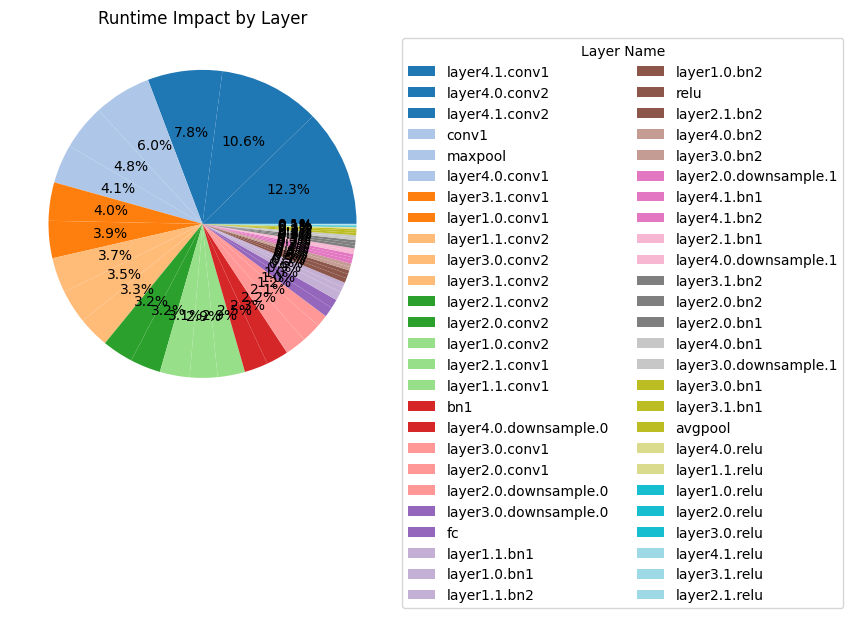
analyzer.layer_wise_impact(ProfilerMetric.RUNTIME).head(5)

[10]:

	ProfilerMetric.NAME	ProfilerMetric.TYPE	ProfilerMetric.RUNTIME	ProfilerMetric.RUNTIME (%)
46	layer4.1.conv1	Conv2d	0.003787	12.306214
42	layer4.0.conv2	Conv2d	0.003270	10.627319
49	layer4.1.conv2	Conv2d	0.002408	7.825804
1	conv1	Conv2d	0.001853	6.021399
4	maxpool	MaxPool2d	0.001475	4.791862

Filter layers by type#

The filter_by_layer_type method can be used to filter the layers by their type. It takes the layer type as an argument and returns a pandas.DataFrame object with the layers of the specified type. Note that all analyzer methods also take a keyword argument readable which can be set to True to return metrics in a human-readable format.

[11]:

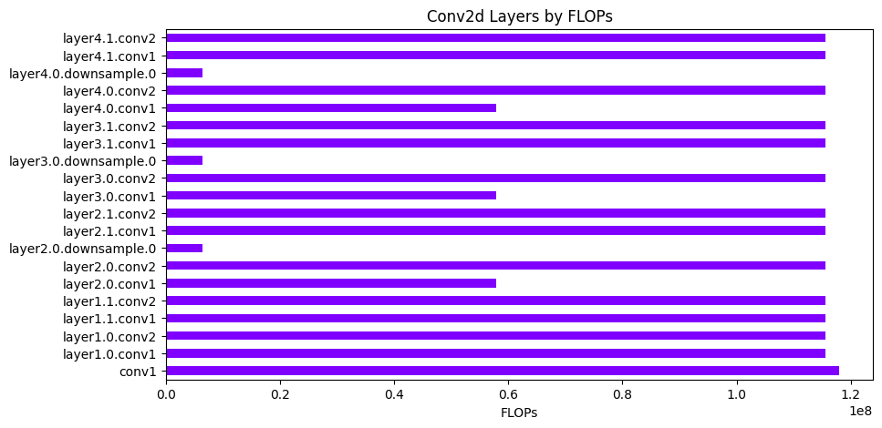
analyzer.find_layers_by_type("Conv2d", readable=True)

[11]:

	ProfilerMetric.NAME	ProfilerMetric.TYPE	ProfilerMetric.INPUTS	ProfilerMetric.OUTPUTS	ProfilerMetric.PARAMS	ProfilerMetric.PARAMS_TRAINABLE	ProfilerMetric.FLOPS	ProfilerMetric.MADDS	ProfilerMetric.MEM_READ	ProfilerMetric.MEM_WRITE	ProfilerMetric.RUNTIME	ProfilerMetric.RMS
1	conv1	Conv2d	(3, 224, 224)	(64, 112, 112)	9.41K	9.41K	118.01M	235.23M	159.94K	802.82K	0.0019	tensor(0.1297)
5	layer1.0.conv1	Conv2d	(64, 56, 56)	(64, 56, 56)	36.86K	36.86K	115.61M	231.01M	237.57K	200.7K	0.0012	tensor(0.0535)
8	layer1.0.conv2	Conv2d	(64, 56, 56)	(64, 56, 56)	36.86K	36.86K	115.61M	231.01M	237.57K	200.7K	0.001	tensor(0.0452)
10	layer1.1.conv1	Conv2d	(64, 56, 56)	(64, 56, 56)	36.86K	36.86K	115.61M	231.01M	237.57K	200.7K	0.0009	tensor(0.0509)
13	layer1.1.conv2	Conv2d	(64, 56, 56)	(64, 56, 56)	36.86K	36.86K	115.61M	231.01M	237.57K	200.7K	0.0011	tensor(0.0440)
15	layer2.0.conv1	Conv2d	(64, 56, 56)	(128, 28, 28)	73.73K	73.73K	57.8M	115.51M	274.43K	100.35K	0.0006	tensor(0.0416)
18	layer2.0.conv2	Conv2d	(128, 28, 28)	(128, 28, 28)	147.46K	147.46K	115.61M	231.11M	247.81K	100.35K	0.001	tensor(0.0340)
20	layer2.0.downsample.0	Conv2d	(64, 56, 56)	(128, 28, 28)	8.19K	8.19K	6.42M	12.74M	208.9K	100.35K	0.00038	tensor(0.0707)
22	layer2.1.conv1	Conv2d	(128, 28, 28)	(128, 28, 28)	147.46K	147.46K	115.61M	231.11M	247.81K	100.35K	0.0009	tensor(0.0342)
25	layer2.1.conv2	Conv2d	(128, 28, 28)	(128, 28, 28)	147.46K	147.46K	115.61M	231.11M	247.81K	100.35K	0.001	tensor(0.0301)
27	layer3.0.conv1	Conv2d	(128, 28, 28)	(256, 14, 14)	294.91K	294.91K	57.8M	115.56M	395.26K	50.18K	0.0007	tensor(0.0291)
30	layer3.0.conv2	Conv2d	(256, 14, 14)	(256, 14, 14)	589.82K	589.82K	115.61M	231.16M	640.0K	50.18K	0.0011	tensor(0.0251)
32	layer3.0.downsample.0	Conv2d	(128, 28, 28)	(256, 14, 14)	32.77K	32.77K	6.42M	12.79M	133.12K	50.18K	0.00032	tensor(0.0330)
34	layer3.1.conv1	Conv2d	(256, 14, 14)	(256, 14, 14)	589.82K	589.82K	115.61M	231.16M	640.0K	50.18K	0.0012	tensor(0.0224)
37	layer3.1.conv2	Conv2d	(256, 14, 14)	(256, 14, 14)	589.82K	589.82K	115.61M	231.16M	640.0K	50.18K	0.001	tensor(0.0207)
39	layer4.0.conv1	Conv2d	(256, 14, 14)	(512, 7, 7)	1.18M	1.18M	57.8M	115.58M	1.23M	25.09K	0.0013	tensor(0.0199)
42	layer4.0.conv2	Conv2d	(512, 7, 7)	(512, 7, 7)	2.36M	2.36M	115.61M	231.19M	2.38M	25.09K	0.0033	tensor(0.0174)
44	layer4.0.downsample.0	Conv2d	(256, 14, 14)	(512, 7, 7)	131.07K	131.07K	6.42M	12.82M	181.25K	25.09K	0.0007	tensor(0.0328)
46	layer4.1.conv1	Conv2d	(512, 7, 7)	(512, 7, 7)	2.36M	2.36M	115.61M	231.19M	2.38M	25.09K	0.0038	tensor(0.0180)
49	layer4.1.conv2	Conv2d	(512, 7, 7)	(512, 7, 7)	2.36M	2.36M	115.61M	231.19M	2.38M	25.09K	0.0024	tensor(0.0132)

Analyze memory usage#

The analyze_memory_usage method can be used to analyze the memory usage of the model. It returns a pandas.DataFrame object with the memory usage of each layer.

[12]:

analyzer.analyze_memory_usage(readable=True).head(
    5
)  # only first 5 layers (for brevity)

[12]:

	ProfilerMetric.NAME	ProfilerMetric.MEM_READ	ProfilerMetric.MEM_WRITE
1	conv1	159.94K	802.82K
2	bn1	802.94K	802.82K
3	relu	802.82K	802.82K
4	maxpool	802.82K	200.7K
5	layer1.0.conv1	237.57K	200.7K

Plotting the results#

This section is under construction

[13]:

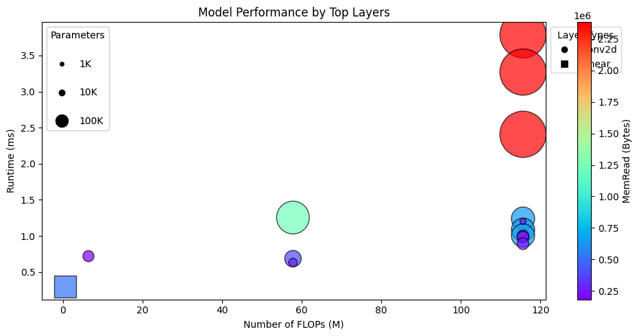
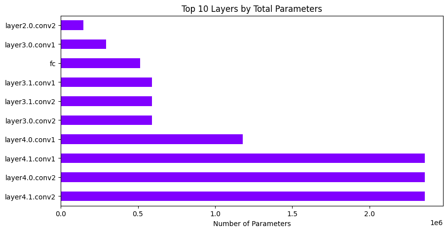
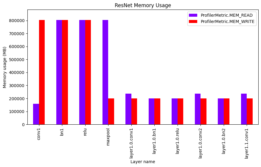
figsize = (10, 5)
analyzer.plot_top_n_layers(n=15, figsize=figsize, colormap="rainbow").show()
analyzer.plot_total_params_per_layer(
    figsize=figsize, colormap="rainbow", limit=10
).show()
analyzer.plot_memory_usage(figsize=figsize, colormap="rainbow").show()
analyzer.plot_layer_wise_impact(
    ProfilerMetric.RUNTIME, figsize=figsize, colormap="tab20"
).show()
analyzer.plot_layers_by_type(
    "Conv2d", metric=ProfilerMetric.FLOPS, figsize=figsize, colormap="rainbow"
).show()

../../_images/nervai-optim_profiling_tutorial_1_22_0.png

../../_images/nervai-optim_profiling_tutorial_1_22_1.png

../../_images/nervai-optim_profiling_tutorial_1_22_2.png

../../_images/nervai-optim_profiling_tutorial_1_22_3.png

../../_images/nervai-optim_profiling_tutorial_1_22_4.png